nbconv

Introduction

The negative binomial (NB) distribution is widely used to model count data whose variance is greater than expected given other discrete probability distributions. The ability to account for overdispersion in observed data using the NB distribution has led to its application across a wide range scientific disciplines as an alternative to Poisson models. Recently, I was interested in evaluating the sum of independent but not identically distributed negative binomial random variables (r.v.s). I discovered relatively quickly, however, that a straightforward solution to this problem doesn’t really exist. The exact solutions that have been published by Furman and Vellaisamy both have significant computational drawbacks. Approximate methods have also been described for such sums, which largely alleviate the computational burdens of the exact methods, but at the potential cost of numeric accuracy. What really befuddled me, however, was the fact that I was unable to find any widely accessible package/tool/etc. that would let me easily apply any/all of these methods to actual data. As such, I wrote the R package that I felt was missing: nbconv.

The current version of nbconv can be found on CRAN and the developmental version can be found on GitHub.

Package description

nbconv was written with the same general syntax as other distribution functions in R. The package has 5 principal functions: dnbconv(), pnbconv(), qnbconv(), rnbconv(), and nbconv_params(). The first four of these return the mass function (PMF), distribution function (CDF), quantile function, and random deviates, respectively, for the convolution of NB r.v.s. The function nbconv_params() returns summary statistics of a given NB convolution based on its moments. The signatures for the 5 principal functions are:

dnbconv(counts, mus, ps, phis, method = c("exact", "moments", "saddlepoint"), 
n.terms = 1000, n.cores = 1, tolerance = 1e-3, normalize = TRUE)

pnbconv(quants, mus, ps, phis, method = c("exact", "moments", "saddlepoint"),
n.terms = 1000, n.cores = 1, tolerance = 1e-3, normalize = TRUE)

qnbconv(probs, counts, mus, ps, phis, method = c("exact", "moments", "saddlepoint"),
n.terms = 1000, n.cores = 1, tolerance = 1e-3, normalize = TRUE)

rnbconv(mus, phis, ps, n.samp, n.cores = 1)

nbconv_params(mus, phis, ps)

The parameterization of the NB distribution used in nbconv is the same as the parameterization used by stats::d/p/q/rnbinom(). All of the nbconv functions take as input vectors of either constituent distribution means (mus) or probabilities of success (ps) and consitutent distribution dispersion parameters (phis, referred to as size in stats).

The PMF, CDF, and quantile functions all require specification of the evaluation method. In nbconv, these are: Furman’s exact equation (method = “exact”), a method of moments approximation (method = “moments”), and the saddlepoint approximation (method = “saddlepoint”). I’ll avoid the gory mathematical details of the evaluation methods in this post, but a detailed description can be found here. To give credit where it is due, Martin Modrák’s blog post was my inspiration to include the saddlepoint approximation in nbconv.

Other method-specific variables can also be user-defined in these functions. The variables n.terms and tolerance only pertain to evaluation via Furman’s exact function and define 1) the number of terms included in the series and 2) how close the sum of the PMF of the mixture r.v. $K$ (see the method descriptions) must be to 1 to be accepted, respectively. The threshold defined via tolerance serves as a way to ensure that the number of terms included in the series sufficiently describe the possible values of $K$. The variable normalize pertains to evaluation via the saddlepoint approximation and defines whether or not the saddlepoint density should be normalized to sum to 1, since the saddlepoint PMF is not guaranteed to do so. Evaluation of the mass, distribution, and quantile functions via the exact or the saddlepoint methods, as well as generation of random deviates via rnbconv(), can be parallelized by setting n.cores to a value greater than 1. It should be noted, however, that for the exact function, only evaluation of the PMF, and evaluation of the recursive parameters, are parallelized. Because of this, CPU time for evaluation of the exact function is linearly related to the number of terms included in the series. rnbconv() and nbconv_params() work independently of the evaluation methods described above. The variable n.samp in rnbconv() defines the number of random deviates to be sampled from the target convolution.

Examples

To demonstrate general use of nbconv functions, I’ll generate some sample data. I’ll use the gamma distribution to ensure that $\mu ≥ 0$ and $\phi > 0$.

library(nbconv)

set.seed(1234)
mus <- rgamma(n = 25, shape = 3.5, scale = 3.5)

set.seed(1234)
phis <- rgamma(n = 25, shape = 2, scale = 4)

Summary statistics of the convolution can be informative as to what methods might or might not work well with our data. I won’t go into too much detail here, but in general, the exact method provides the most accurate results but at what can be a steep computational cost. For convolutions of wildly different NB distributions and/or highly overdispersed distributions, the influence of the mixture distribution on the shape of the convolution grows. When this happens, the number of terms included in the series generally has to increase as well. Because the exact method depends on recursive parameters, this means linearly increasing computation time. However, in instances where the convolution is largely symmetric and/or doesn’t exhibit a large degree of kurtosis, the method of moments and saddlepoint approximations work pretty well. Anecdotally, the saddlepoint approximation is a little bit more robust to skewness and kurotosis than the method of moments approximation, but I won’t explore this point in any more detail here.

nbconv_params( mus = mus, phis = phis )
#>         mean       sigma2     skewness  ex.kurtosis       K.mean 
#> 259.98524927 722.99508196   0.17586635   0.04909827  26.26988006

The output of nbconv_params() tells us that the convolution of the sample NB r.v.s is approximately symmetric and doesn’t exhibit much tailing. Because of this, we could probably get away with using any of the three evaluation methods. For the purposes of demonstration, however, I’ll go ahead and use them all. I’ll additionally calculate empirical probability masses from random deviates sampled using rnbconv() to serve as reference data.

samps <- rnbconv( mus = mus, phis = phis, n.samp = 1e6, n.cores = 1 )

empirical <- stats::density(x = samps, from = 0, to = 500, n = 500 + 1)$y

exact <- dnbconv( mus = mus, phis = phis, counts = 0:500, 
                  method = "exact", n.terms = 1000, n.cores = 1 )

moments <- dnbconv( mus = mus, phis = phis, counts = 0:500, method = "moments" )

saddlepoint <- dnbconv( mus = mus, phis = phis, counts = 0:500, 
                        method = "saddlepoint", n.cores = 1, normalize = TRUE )

For easier visualization, I’ll combine the four calculated probability mass vectors into a single long data frame.

df <- data.frame( empirical, exact, moments, saddlepoint )

df$count <- c( 0:500 )

df <- df |>
  tidyr::pivot_longer( cols = !count, names_to = "method", values_to = "probability") |>
  dplyr::arrange( method, count )

df$method <- factor( df$method, levels = c("empirical", "exact", "moments", "saddlepoint") )

library( ggplot2 )

ggplot(data = df,
       aes(x = count, y = probability , fill = method ) ) +
  geom_area(data = df[df$method == "empirical",],
            aes(x = count, y = probability ),
            color = "gray50", fill="gray50",
            inherit.aes = FALSE, alpha = 0.5 ) +  
  geom_point(shape = 21, size = 2, color = "#00000000") +
  scale_fill_manual(values = c("gray50","darkblue","darkred","darkgreen"),
                     labels = c("Empirical", "Exact", "Moments", "Saddlepoint" ),
                     guide = guide_legend(title.position = "top",
                                          title.hjust = 0.5,
                                          override.aes = list( size = 2.5 ) ) ) +
  theme_bw() +
  theme(axis.title = element_text(size = 16),
        axis.text = element_text(size = 14),
        legend.position = "top",
        legend.title = element_blank(),
        legend.key.size = unit(3, "point"),
        panel.spacing = unit(1, "lines") ) +
  labs(x = "Counts", y = "Probability")

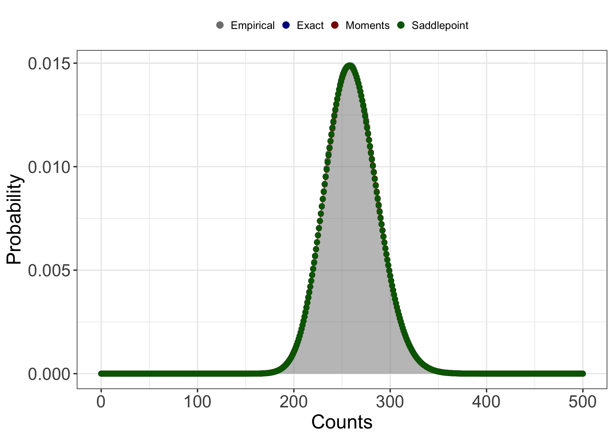
Visualizing the data, we can see that all three methods do indeed appear describe the empirical distribution well. This will not always be the case! I strongly encourage users of nbconv to pay attention to the summary statistics of the target convolution and to compare the evaluated distribution to random deviates!

Hopefully this brief example effectively demonstrates the general workflow of nbconv. If you have any comments or questions, please reach out!