calibrateR

Introduction

When working at the bench, there are probably certain experiments and/or calculations that you routinely do that you hate doing. There’s no logical reason for why you feel this way. The experiment/calculation isn’t hard per se, you just wish that you didn’t have to do it again.

With this feeling of frustration in mind, I decided to streamline some of these common calculations so that the heavy lifting is done behind the scenes (insofar as there is anything truly “heavy” about these calculations – perhaps “the clicking-and-dragging” is more apt). The result, calibrateR, is an easy-to-use R package that contains functions to help with Gibson assembly reaction setup, protein concentration determination via colorimetric assays, size exclusion column calibration, and more. I am happy to expand calibrateR’s current functionalities. Please reach out with other ideas/suggestions!

calibrateR can be downloaded from GitHub.

Usage

library(calibrateR)

Colorimetric Assays

I’ll start by describing the way that the package approaches colorimetric assays. For those who might be unfamiliar, colorimetric assays are a very common way of determining the concentration of analytes in solution. There are various types of colorimetric assays, but the general procedure is similar across the board. First, the user must calibrate the assay by measuring the output signal across a range of known analyte concentrations. Then, from the empirically determined relationship between analyte concentration and signal, the concentration of analyte in the experimentally relevant samples can be determined.

In the example below, I start with defined standard analyte concentrations (conc) and three replicates (rep1-3) of corresponding signal readings. Note that the signal readings are entered in the same order as the known concentrations.

conc <- c(2, 1.5, 1, 0.75, 0.5, 0.25, 0.125, 0.025, 0)
rep1 <- c(2.312, 1.786, 1.273, 1.035, 0.744, 0.484, 0.351, 0.237, 0.209)
rep2 <- c(2.249, 1.739, 1.207, 0.984, 0.701, 0.455, 0.338, 0.23, 0.209)
rep3 <- c(2.282, 1.715, 1.204, 0.99, 0.712, 0.484, 0.345, 0.24, 0.208)

Next, I will use the calibrate_colorimetric() function in calibrateR to create a new function, here called bca(), to do all of the downstream data analysis for me.

bca <- calibrate_colorimetric( conc = conc,
                               abs = c( rep1, rep2, rep3 ),
                               with.blank = TRUE,
                               nrep = 3 )

With the calibrated function defined, we can do one of two things. The first thing we should do is look at our fit and make sure it’s reasonable. To do this, we’ll use our concentration values to calculate expected signal values based on the fit parameters. To do this, call bca( a = conc, return.conc = FALSE ). In this instance, we enter the known concentration values, and tell the function that it is not returning concentration values (it’s returning signal values). Because the units of both concentration and signal can vary widely across assays, I intentionally left units off of the example plot.

library( ggplot2 )

bca.df <- data.frame( conc = conc,
                      meas = c( rep1, rep2, rep3 ) )

bca.fit.df <- data.frame( conc = conc, 
                          fit = bca( a = conc, return.conc = FALSE ) )

ggplot( bca.df, aes( x = conc, y = meas ) ) +
  geom_point(shape = 21, color = "black", fill = "gray75", size = 2.5) +
  geom_line( data = bca.fit.df, aes( x = conc, y = fit ), color = "red", linewidth = 0.75 ) +
  theme_bw() + 
  theme( axis.text = element_text( size = 14 ),
         axis.title = element_text( size = 16 ) ) +
  labs( x = "Concentration", y = "Signal" )

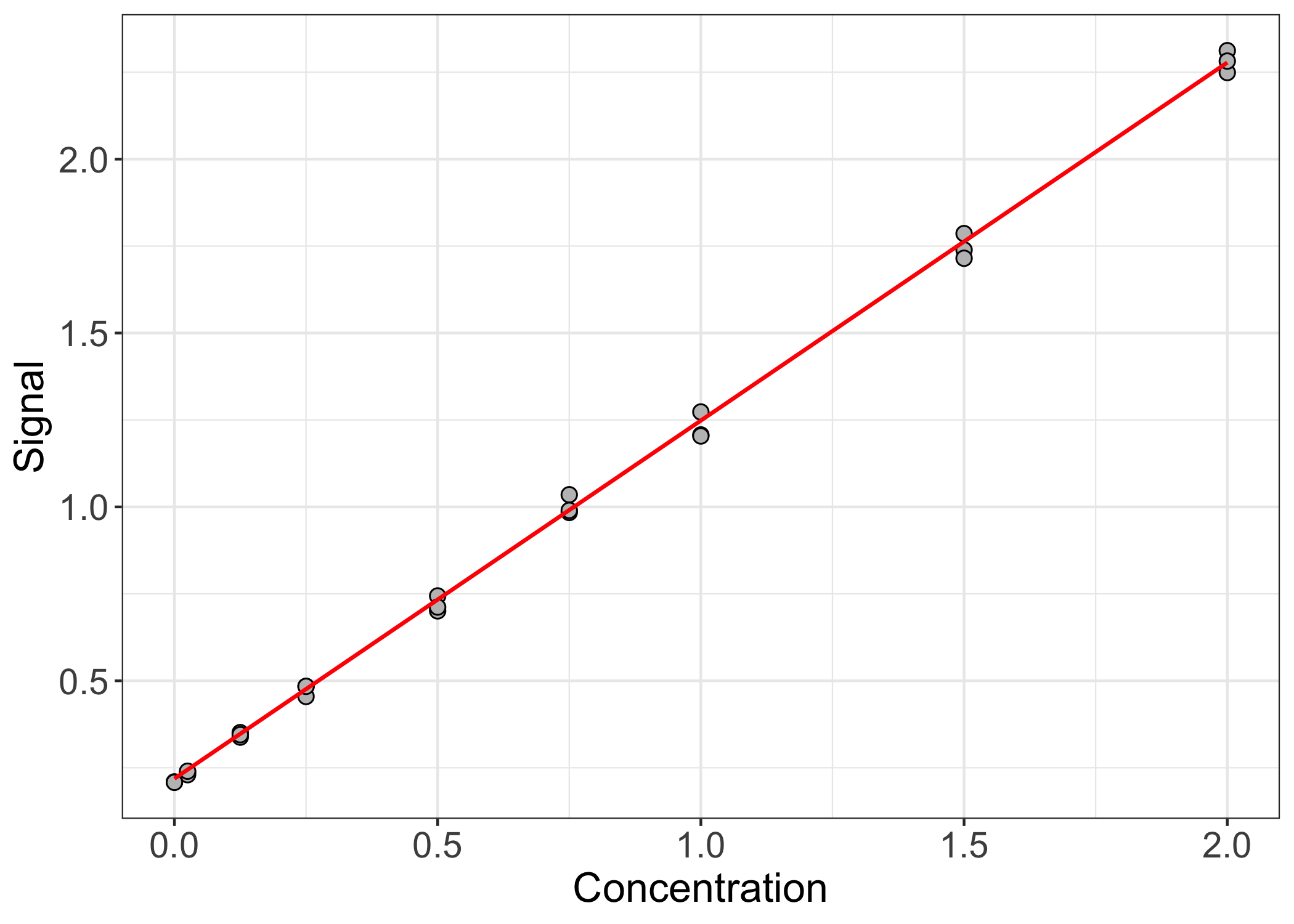The fit seems reasonable. The observed data points lie nicely along the fitted line. Now that we’ve calibrated the assay and are fairly confident that the calibration makes sense, we can feed in signal values from samples of unknown concentration. Here, we’ll assume that we have five unknown samples and that each unknown sample was measured at a 2-fold dilution. We will use return.conc = TRUE and df = 2 in bca() to tell the function that it is returning concentration values and to define the dilution factor(s), respectively. The returned units of concentration are the same as the units of concentration used to make the standard curve.

set.seed( 1234 )
unk <- runif(5, min = 0.3, max = 2)

bca( a = unk, return.conc = TRUE, df = 2 )
#> [1] 0.5453686 2.2248925 2.1818814 2.2284591 3.0128681

Gibson assembly

To calculate Gibson assembly reaction volumes, you need to define eight parameters for each reaction. These are: insert concentration(s), insert length(s), vector concentration, vector length, the number of fragments in the reaction, the molar ratio of insert to vector, the mass of vector in the reaction (in ng), and the final volume of the reaction before the addition of 2x master mix. Concentration units should be ng/µL (or equivalent) and length units should be bp.

The function can calculate parameters for multiple reactions one fell swoop. Vectors with lengths corresponding to the number of unique reactions must be entered for all parameters except insert concentration and insert length. For each reaction, the function will then extract the relevant parameters from the input vectors and perform the requisite calculations. A list of data frames is returned, where each list element represents a unique reaction.

In the example below, I’m calculating reaction parameters for two reactions. The first reaction has 2 input fragments and the second has 3.

gibson( insert.conc = c( 35, 78, 48, 37, 40 ), 
        insert.len = c( 1894, 2403, 887, 1764, 943 ),
        vec.conc = c( 55, 65 ), 
        vec.len = c( 4710, 5934 ), 
        n.frag = c( 2, 3 ), 
        vec.mass = rep( 50, 2 ),
        molar.ratio = rep( 3, 2 ), 
        final.vol = rep( 5, 2 ), 
        ids = c( "Reaction 1", "Reaction 2" ) )
#> $`Reaction 1`
#>            Volume
#> Fragment 1   1.72
#> Fragment 2   0.98
#> Vector       0.91
#> Water        1.39
#> Master Mix   5.00
#> 
#> $`Reaction 2`
#>            Volume
#> Fragment 1   0.47
#> Fragment 2   1.21
#> Fragment 3   0.60
#> Vector       0.77
#> Water        1.95
#> Master Mix   5.00

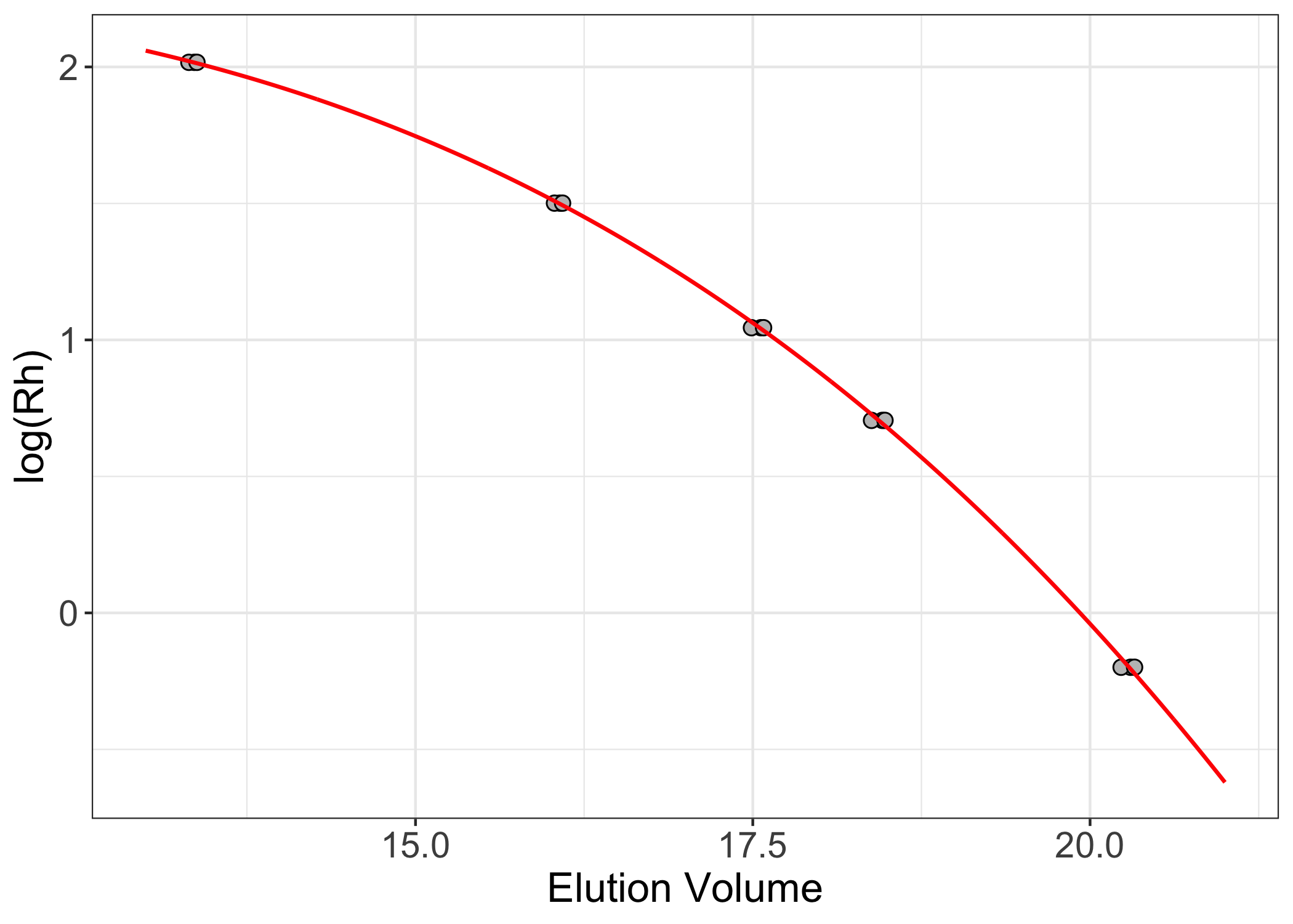
Size exclusion column calibration

Size exclusion chromatography (SEC) is a wildly available technique that can provide useful information about macromolecules. Most commonly, SEC is associated with molecular weight. However, SEC actually separates macromolecules according to their hydrodynamic radius (or Stokes radius). For macromolecules with similar overall shapes, changes in hydrodynamic radius are due predominantly to changes in the number of atoms present in the molecule (i.e., its mass). For macromolecules of different shapes, however, separation based on hydrodynamic radius is a poor indicator of molecular weight. For this reason, it is important to be able to calibrate SEC columns for both radius and mass.

The calibrate_sec() function in calibrateR works similarly to the calibrate_colorimetric() function described above. The function minimally requires the user to define three parameters: the measured elution volume of standard analytes, the masses (yes, just the masses; in Da) of standard analytes, and the macromolecular parameter of interest – either molecular weight (mw) or hydrodynamic radius (rh).

masses <- c( 670000, 158000, 44000, 17000, 1350 )
rep1 <- c( 13.36, 16.07, 17.56, 18.46, 20.30 )
rep2 <- c( 13.32, 16.03, 17.49, 18.38, 20.23 )
rep3 <- c( 13.38, 16.09, 17.58, 18.48, 20.33 )

sec.rh <- calibrate_sec( vols = c( rep1, rep2, rep3 ),
                         masses = masses,
                         parameter = "rh" )

Running calibrate_sec() returns a function for downstream number crunching. Setting parameter = “rh” uses a previously published scaling law to convert the provided mass values to radius values.

Convention for SEC column calibration plots is to plot $\log{(M)}$ or $\log{(R_H)}$ vs. volume. Here, I will create a sequence of dummy elution volumes between the observed elution volumes for the standard analytes. Because I calibrated the column based on hydrodynamic radius instead of mass, I will use the function mass_to_radius() to convert the standard analyte masses to hydrodynamic radii. Then, I will use the calibration to calculate the expected radii of analytes eluting at each of the dummy elution volumes. Non-normalized elution volumes are typically entered in mL units. Because these units don’t strictly matter, however, I’ve left those units off of the plot. The y-axis values are log-transformed. By default, however, the function automatically re-transforms the expected values to the linear scale. Note that the input mass units must be g/mol (Daltons). Calculated mass values are returned in the same units. Hydrodynamic radius values are returned in nm.

sec.df <- data.frame( vols = c( rep1, rep2, rep3 ),
                      rads = mass_to_radius( masses = masses ) )

sec.fit <- data.frame( vols = seq( 13, 21, 0.01 ),
                       fit = sec.rh( seq( 13, 21, 0.01 ) ) )

ggplot( sec.df, aes( x = vols, y = log( rads ) ) ) +
  geom_point(shape = 21, color = "black", fill = "gray75", size = 2.5) +
  geom_line( data = sec.fit, aes( x = vols, y = log( fit ) ), color = "red", linewidth = 0.75 ) +
  theme_bw() + 
  theme( axis.text = element_text( size = 14 ),
         axis.title = element_text( size = 16 ) ) +
  labs( x = "Elution Volume", y = "log(Rh)" )

To apply the calibrated function to analytes of unknown mass/radius, simply enter the empirical elution volume of the analyte into the function. If the column calibration was done using normalized elution volumes, the function normalize_ev() will normalize the analyte elution volumes based on the column’s void and column volumes.

sec.rh( 16.495 )
#>      a 
#> 3.9831

UV/Vis

Concentration determination by UV/Vis spectroscopy is very common in the lab. The calibrateR function uv_vis() takes as input the measured absorbance at the desired wavelength, the extinction coefficient of the molecule of interest, the dilution factor of the measurement, the path length of light, and the type of molecule being measured. If the type of molecule being measured is “protein”, the extinction coefficient must be defined. If the type of molecule is one of dsDNA, ssDNA, or ssRNA, the extinction coefficient can be NULL, and the standard (average) extinction coefficients for these macromolecules are used. The path length defaults to 1 cm.

In the example below, a two-fold dilution of a purified protein with an extinction coefficient of 35000 M^-1cm^-1 was measured to have an absorbance of 0.491 at 280 nm. uv_vis() returns concentrations in same concentration units used in the extinction coefficient. In the example, that is molar units.

uv_vis( abs = 0.491, 
        ext = 35000,
        df = 2,
        type = "protein" )
#> [1] 2.805714e-05